Rediscovering Fourier
My university degree was in Electrical Engineering and naturally the topic of Fourier series and transforms came up frequently throughout different courses.
I have a confession to make though.
Even though I sailed through my degree and could regurgitate the formulas and pass the exams, I never truly “got” what a Fourier Series was or what a Fourier Transform did. I never thought I would need to use it anyways since the applications I was shown were always related to Sound or Signal Processing.
It came as a surprise for me then when I started delving into Data Science and Machine Learning how ubiquitous the Fourier Trasnform and Series were. For example, in Deep Learning the Convolution layers are done in the frequency domain [3] since this makes the operation significantly more efficient. In forecasting, it seems to be quite common to use Fourier series to represent some seasonal/periodic effect on the time series [4].
After brushing over the details for these implementations, I decided to actually re-visit Fourier and attempt to really get it this time.
Inner product of Functions
I spent some time to go through Professor Brunton’s book and videos on Fourier Analysis [1,2]. What I found really useful was his interpretation of the Fourier Series using a Linear Algebra/Geometric view.
We can view the Fourier series as an inner product of functions between the function \(f(x)\) we are attempting to reproduce and various sines and cosines of different frequencies. Let me try to explain using the image below.
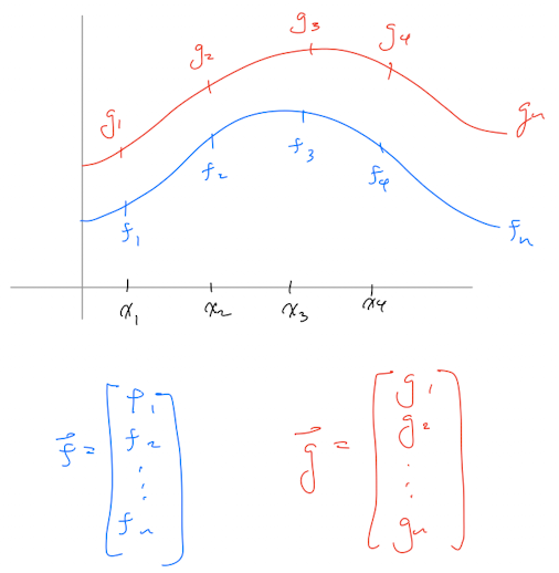
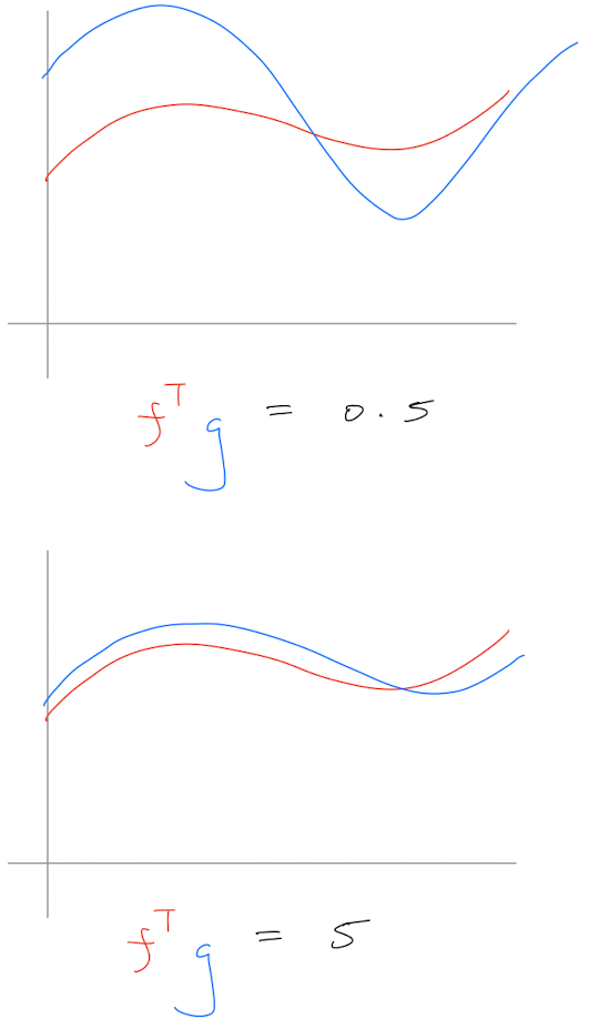
\(\vec{f}\) and \(\vec{g}\) are outputs for two functions given the same inputs. If we plot the inputs and outputs, we would get something similar to the plot above. Intuitively, we could reason that if the two lines in the plot are quite similar or even overlapping this must mean the two functions must also be similar. Quantitatively we can calculate the inner-product between these two vectors as \(f^{T}g\). The higher their “similarity”, the larger the inner-product and vice versa.
Fourier Series is an inner product between the function and sin/cos
Fourier Series can be interpreted as using a collection of sines and cosines to represent a function. In Linear Algebra speak, we use sines and cosines as the basis and discretise the function on fixed frequencies. The Fourier series formula:
\(f(x)=\frac{A_{0}}{2}+\Sigma_{k}^{inf}(A_{k}cos(kx)+B_{k}sin(kx))\)
\(k: frequency\)
\(A_{k}=\frac{1}{\pi}\int_{-\pi}^{\pi}f(x)cos(kx)dx\)
The \(A_{k}\) coefficient represents the inner product between \(f(x)\) and \(cos(kx)\)
\(B_{k}=\frac{1}{\pi}\int_{-\pi}^{\pi}f(x)sin(kx)dx\)
The \(A_{k}\) coefficient represents the inner product between \(f(x)\) and \(sin(kx)\)
The \(\frac{1}{\pi}\) acts as a normalisation term
So in essense, we use a collection of sines and cosines functions to represent our function and the coefficients for any given sine or cosine function is simply how inner product between that particular sine function at a given frequency to our actual function we want to reproduce. If a particular frequency of sine or cosine is “similar” to our function, the coefficient for that particular sine or cosine would be larger compared to one that is not.
We can also interpret this geometrically like below:
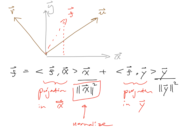
Where our function is \(\vec{f}\) and \(\vec{u}\) and \(\vec{v}\) are two orthogonal functions (just like Sin and Cos). The inner product can be thought of as the “projection” of \(\vec{f}\) onto either \(\vec{u}\) or \(\vec{v}\). The constant term \(\frac{\vec{x}}{\Vert{x}\Vert_{2}}\) at the end just ensures this scales down to a unit vector (normalise in a sense).
This was kind of the “ah-ha, I get it” moment for me. Sometimes staring and rote learning formulas will help you pass tests but I’ve always been more of a visual learner. Professor Brunton’s materials on Fourier Analysis really helped me actually understand it intuitively and I’m grateful he’s made the materials available online free of charge, go check it out.
link to his book online
References:
[1] Fourier Series: Part 1 [https://youtu.be/MB6XGQWLV04] by S.Brunton 2020
[2] Data-Driven Science and Engineering, Brunton & Kutz. Chapter 2
[3] Convolution theorem, Wikipedia. [https://en.wikipedia.org/wiki/Convolution_theorem]
[4] Bayesian Forecasting and Dynamic Models, M.West & J.Harrison. 1999