Bayesian Regression Model (Part 2)
In part 1 of the Bayesian Regression Model, I covered how the traditional OLS interpretation of regression is obtained. I followed this up with an example of the short coming in terms of the predictive uncertainty and how the OLS model may be over confident in predictions even when it has no data to support its claims. In this post, I will explain the Regression model through a Bayesian lens. Highlighting the important difference between OLS and Bayesian Regression in how the solution is arrived at and how the key idea of predictive uncertainty surfaces from this alternative path.
Part 1: Normal OLS Model
Part 2: The Bayesian Lens (This post)
Part 3: Posterior Calculation
Part 4: Bayesian Advantage
Viewing Regression through a Bayesian lens When I first looked into Bayesian Regression models it was one of the most daunting experience for me in my ML journey. Looking back, I think there are two main reasons that contributed to this:
- You need to have some idea of Gaussian distributions in order to understand the reasoning behind a Bayesian Regression model.
- The iterative, sequential nature of the so called posterior calculation is foreign compared to the batch nature of OLS.
The main idea/difference for a Bayesian Regression model is that instead of looking for one single number to represent your coefficient/weight, you are now instead finding a distribution represented by a Gaussian. Since a Gaussian can be summarized by their sufficient statistics, the mean and variance. When making a prediction you will use the mean as your coefficient/weight but now with the added advantage of having a more “realistic” representation of your uncertainty by accounting in your training data.
Now I will cover those two main reasons that I found difficult and hopefully this will help you as well in understanding Bayesian Regression.
Posterior Gaussian conditional
The coefficients are found in OLS using the Moore-Penrose pseudo inverse. This idea is a bit easier to grasp (at least to me) as you can frame it as a Linear Algebra problem where the results \(\hat{y}\) (\(n\times 1\))comes from the matrix multiplication between your data (the design matrix, \(n\times d\)) \(A\) and some unknown weight vector \(x\) (\(d\times 1\)). Since both the input data/independent variable and response/dependent variable are known and only the weights are unknown, we go from \(Ax=b\) to \(x=A^{-1}b\). Think of this as simple algebra if you are not familiar with Linear Algebra, if we have for example \(3x=6\), in order to find \(x\) we move 3 over to the RHS \(x=6/3 = 2\). The \(A^{-1}\) has the same meaning as \(1/A\).
Now, if we compare the OLS model and the Bayesian model, what we find is that the Bayesian model does not require the entire dataset in order to find the weights/coefficients. Instead, the Bayesian model sequentially accepts new data and uses the Gaussian conditioning rule to calculate the “latest” weights/coefficients value. This is the part where in most tutorials they will present the Bayesian model update rules which might look like the following from Bishop:
\(\bf m_{N} = \bf S_{N}(\bf S_{0}^{-1}\bf m_{0} + \beta\Phi^{T}\bf t)\)
\(\bf S_{N}^{-1} = \bf S_{0}^{-1} + \beta \Phi^{T} \Phi\)
It took me a while to understand how this formula was derived but essentially this is using the Gaussian conditioning rule (Formula 4.69 from [3]):
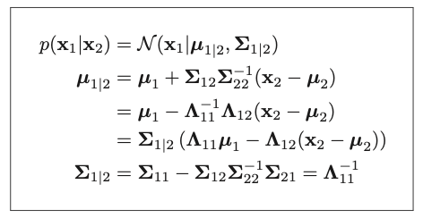
What the formula says, is that if our data are jointly Gaussian (which is the assumption we place and not some empirical proof) than we can update our initial belief of our weights/coefficients (\(u_{1}\) and \(\Sigma_{1}\)) by using the new information from our observed result \(y\).
The exact formula does not look the same and that’s because of the likelihood function for our observation \(p(y|x)\). The derivation of the posterior will be covered in the final part where I will clearly outline how the above Gaussian conditional rule is used in conjunction with the “complete the square” trick to obtain the posterior formula.
References:
[1] Pattern Recognition and Machine Learning, Bishop.
[2] Machine Learning(CPSC-540) Youtube videos, Nando de Freitas. 2013.
[3] Machine Learning, Murphy.