Bayesian Regression Model (Part 1)
Ever since I started working in Data Science and delving deeper into Machine learning models, I have had a strong interest in learning about Bayesian models. It was never really clear to me though why or when a “Bayesian” model would be preferred compared to the more traditional OLS or Tree based models that I was more accustomed to, so there was never really a drive to get serious in learning about it.
I think the turning point came when project stakeholders I was interacting with started asking for some numerical output to represent some representation of our model’s prediction confidence. For a OLS there is the Confidence Interval but the concept never made much sense to me and good luck trying to explain this to a non-technical stakeholder, “…95% of the time our true value lies between this interval…”
This slowly pushed me to look more seriously into Bayesian models where the underlying weights/coefficients were represented as actual probability distributions thus more closely mimicking the way we as humans think of as “confidence”, “Our model is 95% certain this predicted value is correct.”
This topic on Bayesian Regression will be split into multiple parts. I will begin by describing the normal OLS model, this will move to an overview of the Bayesian perspective on Regression and further details on how the posterior for a Bayesian model is calculated. I will also be using one of my project as an example where Bayesian models were able to produce more accurate Regression predictions.
Part 1: Normal OLS Model (This post)
Part 2: The Bayesian Lens
Part 3: Posterior Calculation
Part 4: Bayesian Advantage
Normal OLS Model
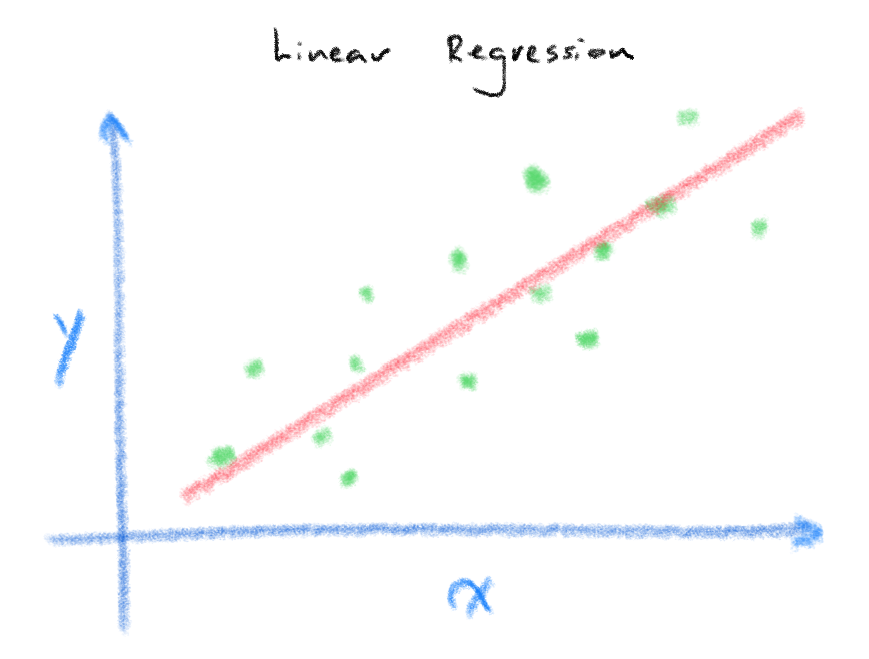
The image above demonstrates a classic example of linear regression where we seek to model the relationship between our input/independent variable \(X\) and our prediction/dependant variable \(y\). In plain speak, we want to find out what is the most likely value of \(y\) given that we know the value of \(X\). A simple but classic example of this is Francis Galton’s Father and Son height dataset where given the height of the father (\(X\)) you could predict the son’s height (\(y\)).
\[y(x,w)=\sum\limits_{j=0}^{M-1} w_{j}\phi_{j}(x) = w^{T} \phi(x)\]Most of us should be quite familiar with the formula above ([1]Formula 3.2)for Linear Regression where you find \(y\) from some combination of scalar weights/coefficients, w multiplied by the \(x\) and you sum this up for all \(w\) and \(x\).
In nearly all instances when we wish to train a Regression model, we have data that includes the x and the y variable. What’s left for the algorithm to do when you execute model.fit() is to find the most “optimal” weight. If we disregard the notion of regularisation for now, the weights are often found by minimizing the squared difference between the prediction, \(\hat{y}\) and the true value \(y\).
We will not go into the entire process for how this is done but for those curious, Bishop’s book covers this in detail in chapter 3. What we do need to understand is that we usually require a sufficient amount of data (what exactly does this mean? I will be writing another post to explain this) in \(x\) which we will call the design matrix or data matrix \(\Phi\) that will allow our model to explain \(y\) in order to find a set of weights. If we frame the Linear regression formula in terms of the linear algebra expression \(Ax=b\) where A is our design matrix, \(x\) is our weights and \(b\) is our \(y\), what we can see is that if \(A\) was square and invertible(full rank) we could find our weights by simply doing \(x=A^{-1}b\). The \(A^{-1}\) or \(\Phi^{-1}\) matrix is commonly referred to as the Moore-Penrose pseudo-inverse of the matrix \(\Phi\) [1].
Most of the time this design matrix is over-determined (n » m) where no solutions exist and therefore requires us to use alternative means to approximate this matrix. Usually this is done with the SVD matrix decomposition (this is what Sklearn Linear Regression uses) in order to approximate an optimal solution for our weights vector \(x\) ([2] Chapter 1).
Once these weights \(w\) are found for each column/feature, to predict a value from a given \(x\) we simply multiply the weight (if we only have a single feature) or in the case of multiple features, calculate the inner-product between the input \(x\) vector and the \(w\) vector.
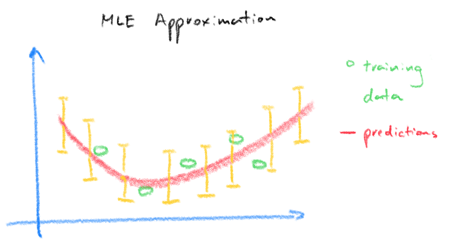
The important result is that the weights found from pseudo-inverse is a point estimate or a single value of the weights, meaning we place no uncertainty on the weights itself but only on the dependant variable. The result is that we place equal uncertainty bounds on our prediction which goes against the intuitive idea that we should be more uncertain of new input test data that are different or further away from the training input data used to find the weights.
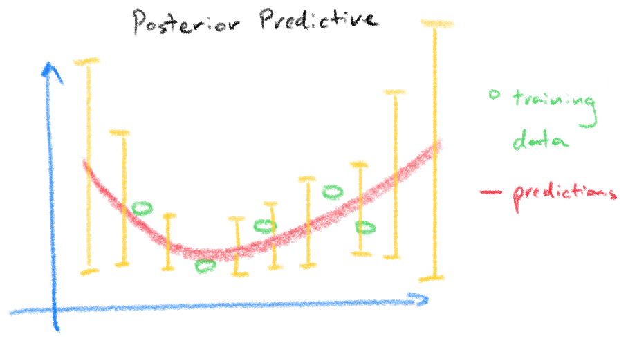
The plots below from [3] demonstrates the idea, the top plot is our result from the pseudo-inverse where the red circles are the training data used to find the weights and the bottom plot is the same data but using a Bayesian regression model where the posterior predictive density takes into account of the uncertainty in the weights reflected in the wider prediction variance for predictions made further away from the training data.
The next part in this series of posts will cover Regression model but this time with a Bayesian perspective. We will see that both the ‘Frequentist’ and ‘Bayesian’ perspective on Regression are fundamentally similar and how the additional complexity added by the Bayesian model gives us additional freedom in modelling our problem.
See you next post!
References:
[1] Pattern Recognition and Machine Learning, Bishop.
[2] Data-Driven Science and Engineering, Brunton & Kutz.
[3] Machine Learning, Murphy.